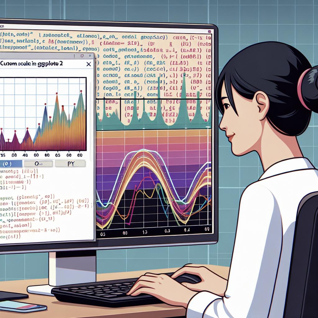
Mastering Custom Scales with ggplot2

In the world of data visualization, ggplot2 in R is a powerful tool that allows for creating intricate and beautiful plots. One crucial aspect of creating informative and visually appealing plots is mastering the customization of scales. This guide explores various ways to manipulate scales in ggplot2, providing examples and insights into tailoring your plots to your specific requirements. We’ll delve into creating time series data, setting axis limits, using specialized scale functions, and transforming data with log and sqrt. Additionally, we’ll address formatting labels and explaining ticks – every detail to ensure your data is presented accurately and effectively.

Example of data

Before diving into custom scales, it’s essential to start with the right kind of data. Typically, in example datasets for ggplot2, you’ll find data frames housing variables that represent different scales. For this tutorial, we will use a simple dataset that features key variables such as ‘date’, ‘value’, and ‘category’.

For instance, consider a dataset tracking stock prices across different companies over time. Each row might include the ‘date’, the ‘closing price’ (our primary variable of interest), and potentially a ‘category’ to distinguish between technology, finance, and healthcare industries. Framing your data correctly sets a solid foundation for applying custom scales with precision.

Create some time series data

Time series data serves as a classic example when illustrating how custom scales can enhance data visualization. Let’s create a simple dataset wherein time – represented by sequential dates – correlates with numeric values. This could represent daily temperatures, stock prices, or any variable changing over time.

In R, creating such a dataset is straightforward: you can use the seq.Date() function to initialize your dates and the runif() function to generate random numeric values. Here’s how you might generate a dataset symbolizing weekly sales data for a company:

dates

spanning over a year, randomly assigned

sales values

, and designated

quarters

as categories.

Plot with dates

When plotting time series data in ggplot2, the key is to set your x-axis to represent time. This involves using ggplot2’s aes() function to establish date as the x component and your variable of interest as the y component.

In our sales dataset example, you’d use ggplot() to create a basic scatterplot with dates on the x-axis. Starting simple, you can then layer in additional components such as geom_line() for continuous lines or geom_point() for distinct data points. This initial stage helps set the groundwork for applying further scale customizations.

Date axis limits

Controlling axis limits is crucial in focusing the narrative of your plot. ggplot2 provides multiple avenues to specify date limits, which allows for zooming in on periods of interest. One such approach is through using the scale_x_date() function, which allows you to directly input the boundaries for your date range.

Alternatively, the xlim() function can be utilized to set date boundaries, although with less precision compared to scale_x_date(). These capabilities ensure that only relevant data is displayed, maintaining the context without unnecessary clutter.

Use xlim() and ylim() functions

xlim() and ylim() functions are vital tools within ggplot2 for controlling plot scales. By defining the minimum and maximum limits on the respective axis, these functions enable you to narrow down your focus on specific data ranges, ultimately enhancing clarity.

These functions are quite efficient for fine-tuning plots, especially when you seek to analyze particular data subsets. For example, when aiming to observe changes solely in the fourth quarter, setting the y-axis to only contain those specific weeks provides a refined view of the dynamics involved.

Use expand_limits() function

Unlike xlim() and ylim(), the expand_limits() function provides a more flexible approach to modifying scales. It’s particularly beneficial when you need to add some padding around data points, ensuring a balanced visual impression without chopping data edges.

For instance, when dealing with financial data, minor fluctuations might be more recognizable with additional whitespace around extreme values. Invoking expand_limits() thus maintains all data points within view while granting your audience a breathable layout.

Use scale_xx() functions

The scale_xx() family of functions extend greater customization that xlim(), ylim() and expand_limits() can’t offer. With scale_x_continuous(), scale_y_continuous(), scale_x_discrete(), and others, you can control the appearance and functionality of your axes’ scales with unprecedented detail.

These include potential log transformations, positioning, and even aesthetic facets such as breaks and minor grid lines, empowering you to dictate how your data narrative unfolds. In data stories where scale representation needs variability or alteration, scale_xx() functions serve as your reliable ally.

Log and sqrt transformations

Transformations using the log and sqrt scales are instrumental in managing data with wide-ranging values. Applying such transformations can reveal important underlying patterns that raw data might obscure.

For instance, using a log transformation can linearize exponential growth patterns, providing clearer insight into trends. Similarly, a square-root transformation might normalize skewed data, offering more balanced insights. ggplot2 allows you to implement these transformations seamlessly through dedicated scale functions like scale_x_log10() and scale_y_sqrt().

Format axis tick mark labels

A crucial aspect of data clarity arises from how we label our plot’s scales. Precise tick mark labels ensure that readers interpret chart data correctly. ggplot2 facilitates this through the scale_x_() and scale_y_() functions, in conjunction with the labels argument, to achieve desired formatting.

Whether you want to append a currency symbol, adjust the date format, or control decimal precision, formatting tick marks can amplify your visualization’s impact. Effective label formatting keeps readers engaged and avoids misinterpretations, exemplifying the details that define rigorous data storytelling.

Display log tick marks

Appropriate tick mark display on log scales contributes to the readability of your plots. Logarithmic scales reduce the gap between massive and minuscule values, making comparisons visual and intuitive, but only if labeled correctly.

ggplot2 offers the functionality to explicitly set these ticks or reverse the display order altogether, accommodating particular narratives or precision requirements. Such fine-tuning allows data to speak directly to its complexity, turning raw numbers into comprehensible patterns.

Recommended for You!

The world of data visualization is vast, and while mastering ggplot2 scales is pivotal, there’s always more to learn. Exploring additional resources can provide deeper insights that build upon the foundation we’ve covered.

Websites focusing on R programming, communities that foster open discussion, or courses that dive into advanced visualization techniques are invaluable. Balancing these resources with practical experimentation accelerates skill advancement and opens doors to new possibilities.

Recommended for you

Books – Data Science

For those looking to dig deeper into data science, the following titles are recommended: “R for Data Science” by Hadley Wickham and Garrett Grolemund, which provides a broad introduction to the field using R.

Additionally, “Data Visualization: A Practical Introduction” by Kieran Healy offers insights tailored for creating informative and compelling visual data narratives. Combining these with your knowledge in ggplot2 will enhance your ability to communicate insights effectively.

Final Thoughts

Key Concept	Details
Data Preparation	Setting up proper datasets, e.g., time series for plots.
Basic Plot Setup	Utilizing ggplot to create foundational visuals with dates.
Axis Limits	Mastering xlim(), ylim(), and scale functions for focus.
Scale Transformations	Log and sqrt transformations for data representation.
Label Formatting	Adjusting tick marks and labels for clear communication.
Resource Exploration	Books and online courses for extended learning.